Teema Studio

Welcome to Teema Studio, an advanced desktop application for PEEC SImulations. This guide will help you familiarize yourself with the interface and make the most of the available tools to create and manage your simulation projects.

Installation & Setup

Docker Requirement

Before starting the application, it is crucial to have Docker installed on your system. The application relies on Docker containers to run the simulation backend efficiently.

Download Docker Desktop

⚠️ Important: Ensure Docker is active/running before launching the application.

CADmIA is a versatile tool for creating 3D models. Initially designed for the electrical/electronic field, it has evolved into a general-purpose modeler. Its modular architecture allows users to combine basic components to build highly complex structures.

Navigating the Scene

Rotate: Click & Drag (Left Mouse)
Pan: Click & Drag (Right Mouse)
Zoom: Mouse Wheel / Touchpad
Focus: View is centered on origin (0,0,0) by default.

Basic Models

Available primitives configurable via SideBar:

CubeSphereCylinderTorusCone

Tip: Adjust radial segments for higher precision or better performance.

Binary Operations & Cloning

Composition

Combine objects using boolean operations. Click to watch examples:

Cloning

Duplicate any object with all current properties to speed up modeling.

Snap-to-face

Snap objects to faces for precise alignment. Click to watch example:

Organization Tools

Essential tools for organizing your scene. Click to watch examples:

Patterning

Create multiple copies of objects in specific arrangements.

Materials

In CADmIA, you can create, manage, and assign custom materials to your objects. This allows for accurate physical simulations by defining specific electromagnetic properties.

Manage Materials

Access the Material Editor to create new materials or modify existing ones. You can define base properties like name and color for visualization.

Physical Properties

Define Permeability, Permittivity, and Conductivity. Each can be set as a constant, or with a Tangent Delta, or as a custom Frequency-Dependent profile.

Material Attributes

Property	Description	Options
General	Basic identification and visualization.	Name, Color
Permeability (μ)	Magnetic property.	Constant, Tangent Delta, Custom (Freq. Dependent)
Permittivity (ε)	Electric property.	Constant, Tangent Delta, Custom (Freq. Dependent)
Conductivity (σ)	Electrical conduction.	Constant, Tangent Delta, Custom (Freq. Dependent)

* Custom properties allow defining Real (Re) and Imaginary (Im) values for specific frequencies.

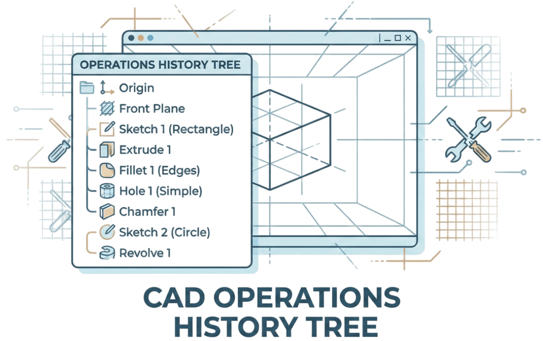
History Tree

Track every operation in your project. Undo/Redo actions or travel back in time to any previous state.

Import / Export

Export

Cloud / Server

Save AsUpload project to server
Save With Ris GeometryInclude rigorous geometry data

Local File System

Export Project (JSON)Full project data
Export STLGeometry mesh only
Export Ris GeometrySeries of cube objects

Import

Cloud / Server

LoadDownload from server

Local File System

Import Ris GeometryFrom local file
A RIS geometry is defined by a series of bricks with specific coordinates.
Each element is defined as:
[Xmin, Xmax, Ymin, Ymax, Zmin, Zmax]
This format cannot be used if the canvas contains complex objects like STLs or geometries resulting from boolean operations.
Format Example: JSON Array of Bricks Sample
Import Project (JSON)Restore full project
Import STLLoad 3D mesh
Sample STL File Sample

ESymIA is a powerful FEM-based simulation tool for analyzing electrical and electronic characteristics of 3D models. The workflow is split into four key stages: Modeler, Physics (Terminations), Simulator, and Results.

Projects Management

The Projects dashboard is your command center in ESymIA. From here, you can create new simulations or open existing ones.

New Project

Start a fresh simulation from scratch. Define your settings and launch your simulation.

Open

Resume work on your saved projects. Access your recent files quickly.

Folder Organization

Organize your projects into logical folders to keep your workspace clean and efficient.

Pro Tip: Project Organization

Use descriptive names for your projects. ESymIA auto-saves your work.

Model Import

Import the 3D model you intend to simulate. You can load your geometry from two primary sources:

FileSystem

Load standard CAD files (JSON) directly from your local computer storage.

Database

Access models stored in the central project database or cloud repository.

Mesher

Discretize your model geometry for simulation. The efficient generation of the mesh is crucial for both accuracy and simulation speed.

Standard Models

For standard geometries, the Uniform Mesher is selected by default.

Set Frequency: input the Max Frequency of your simulation.
Get Quantum: Wait for the system to suggest an optimal Initial Quantum (cell size).
Generate: Create the initial mesh.
Iterate: If the mesh is too coarse or too fine, use the Refine or Coarsen tools to adjust the grid density.

RIS Models

Reconfigurable Intelligent Surfaces (RIS) offer two meshing strategies:

Option A: Uniform

Follows the same workflow as Standard Models (Max Freq → Quantum → Refine/Coarsen).

Option B: Non-Uniform

Set Max Frequency.
Set Lambda Factor (grid scaling).
Generate Mesh.
Adjust parameters and regenerate if needed.

Solver

Configure the physical environment and simulation parameters. This section controls excitations, boundaries, and the time-domain solver settings.

Simulation Type

Select Simulation Mode

Matrix (S, Z, Y)

Compute Scattering, Impedance, and Admittance matrices for multi-port networks.

Electric Fields

Analyze time-domain electric field distribution and propagation in 3D space.

Frequencies

Frequency Settings

Matrix (Z, S, Y)

Define a frequency range by specifying:

Min Value
Max Value
Number of Samples

Or import from CSV:

Sample

Frequencies
1000000
1930697.72...

Electric Fields

Define Final Time and Time Step (in seconds). The frequency range is automatically generated:

function create_freqs(t) { const fintem = t[t.length - 1] - t[0]; const ncampt = t.length; const frefond = 1 / fintem; const f: number[] = []; for (let i = 0; i <= Math.floor(ncampt / 2); i++) { f.push(i * frefond); } return f; }

You can then select specific frequencies to study.

Ports & Plane Waves

Excitations & Sources

Ports

Type: 2D Port (Rect/Circ)
Modes: TE / TM / TEM
Impedance: Auto / User-defined

Lumped Elements

RLC: Resistor, Inductor, Cap
Voltage Src: Signal Generator
Diode: Non-linear models

Plane Waves

Polarization: Linear / Circ / Ellip
Direction: K-Vector (Theta/Phi)
Amplitude: E-field (V/m)

Creation & Import Methods

Ports and lumped elements can be created individually via the graphical interface or imported in batch processing using CSV files.

Ports CSV Format Sample

name, x1, y1, z1, x2, y2, z2, scattering

Lumped Elements CSV Format Sample

name, x1, y1, z1, x2, y2, z2, type, R, L, C

Tip: Positioning Ports & Lumped Elements

There are several ways to set the position of ports:

Double click on the surface
Drag to the desired position
Via numeric input

For greater precision, it is suggested to set the position via numeric input.

Simulation Parameters

Solver Configuration

Solver Type

Rcc Delayed Coefficients

High accuracy computation

Quasi Static Coefficients

Fast approximation

Advanced GMRES Settings

Convergence Threshold1e-4 (DEFAULT)
Stop criterion based on relative residual error.
Inner Iterations1 (DEFAULT)
Maximum number of restart cycles.
Outer Iterations100 (DEFAULT)
Krylov subspace dimension before restart.

Results & Analysis

Visualize your data with the Results viewer. Plot S-parameters, visualize 3D fields, and export data for external processing.

S-Parameters

View Return Loss (S11), Insertion Loss (S21), and Smith Charts. Toggle between Magnitude (dB) and Phase.

3D Fields

Visualize Electric (E) and Magnetic (H) fields on 2D planes or as 3D isosurfaces. Animate fields in time.

Far Field

Compute 3D Radiation Patterns, Gain, Directivity, and Efficiency for antenna designs.

Export formats supported:

.s2p.csv

Storage & Management

Efficiently manage your simulation data. ESymIA handles large field monitors and mesh data with a smart caching system.

Autosave & Recovery

ESymIA includes a robust auto-save feature that snapshots your project on every change.

Sharing Functionalities

Real-time collaboration is not supported. Sharing a project performs a "Clone & Associate" operation: the project is duplicated and linked to the recipient's account. They view it as an independent project and can modify it without affecting your original version.

Cloud Sync

Every project is automatically synchronized to the cloud.

Demo Version Limitations:

Maximum of 3 projects
No folder organization
Sharing features disabled

Data Footprint

Mesh DataHigh

Ports & Lumped ElementsMedium

ResultsLow